
Seasonal Demand Forecasting for Auto Repair Shops
A flat monthly average looks tidy on a spreadsheet. It fails on the shop floor. One week brings dead batteries, no-starts, and tire calls faster than the front desk can answer. The next week brings open bays and technicians waiting for work. Seasonal demand forecasting fixes that mismatch by planning for the week that's coming, not an average week that rarely exists. The goal isn't a perfect prediction. The goal is staffed bays, parts on the shelf, and fewer declined jobs.
Table of Contents
- Why Seasonal Demand Forecasting Matters in the Bay
- Build a Clean Weekly History Before You Forecast
- Choose a Seasonal Method That Fits Shop Data
- Run a Seasonal Index With Shop-Scale Numbers
- Turn the Forecast Into Hours Parts and Capacity
- Review Forecasts When Weather and Demand Shift
- Put Seasonal Demand Forecasting to Work This Week
Why Seasonal Demand Forecasting Matters in the Bay
A shop staffs to last month's average, orders a normal round of batteries and tires, and opens the calendar as usual. Then the first hard cold snap hits, or summer heat exposes weak cooling systems, or inspection deadlines stack up before holiday travel. The phones don't slow down. Advisors squeeze cars between appointments, technicians stay late, and parts that should've been ordered days earlier arrive after the rush has already peaked.

The slow weeks cost money too. Bays sit empty, booked hours fall short, and cash gets tied up in parts bought for a surge that has already passed. Owners often read the busy stretch as growth and add hours permanently, then watch demand settle back to normal. That mistake comes from treating a predictable seasonal spike as a lasting change in the business.
What a Useful Forecast Changes
Good seasonal demand forecasting separates three things: the underlying trend, the recurring seasonal effect, and irregular noise. Classical time-series decomposition does exactly that, and weekly sales research separating trend, seasonal, and irregular components shows why weekly history reveals peaks that annual totals hide. For a repair shop, those peaks usually connect to weather, travel, inspections, holidays, or vehicle-use cycles.
- Staffing decisions: Managers schedule technician-hours for the expected peak instead of reacting with overtime.
- Parts decisions: Batteries, tires, cooling parts, and inspection supplies get ordered before the phones spike.
- Appointment capacity: Advisors protect slots for seasonal work instead of filling the week with jobs that could wait.
- Cash-flow planning: Owners stop mistaking a seasonal surge for permanent growth.
Each location needs its own profile. A northern shop's battery season doesn't match a southern shop's air-conditioning season, and a fleet-heavy location moves differently from a retail location near a highway. Multi-location groups that force one demand curve onto every garage will understaff one shop and overbuy at another. The sections ahead give owners a weekly workflow, a worked index calculation, and a practical way to turn a range of outcomes into bay, staffing, and parts decisions.
Build a Clean Weekly History Before You Forecast
No formula fixes bad records. A forecast built on messy repair orders repeats the mess with more confidence. Owners should start with records the shop already creates and clean them before any calculation begins.
Pull the Records That Reflect Real Demand
The starting set includes appointments, repair orders, parts lines, cancellations, no-shows, and the team calendar. Repair orders show completed work, but cancellations and no-shows matter because booked demand and finished demand aren't the same thing. Parts lines help separate a true service surge from a few large tickets that inflated revenue without filling many bays.
Forecasts should sit at the service-category and weekly level, not only at total monthly revenue. Monthly revenue blends oil changes, diagnostics, tires, batteries, and major repairs into one number that can't drive staffing. Daily tickets are often too sparse to read, so aggregating daily observations into weekly and monthly views helps a real pattern show through the noise.
Regular work also needs separation from rare work. Oil changes and seasonal tire jobs recur often enough for a seasonal pattern. Infrequent specialty repairs don't, and averaging them as if they arrive every week creates phantom demand. Keep intermittent categories in a separate bucket from the start.
Practical rule: A category that appears only occasionally should never be averaged into the weekly plan for oil, tires, batteries, or inspections.
Mark the Calendar and Cap the Freak Weeks
Each week needs context. Owners should add markers for month, week of year, holidays, weather, mileage or vehicle age, and promotions. A promotion can lift demand once, but it isn't seasonality, and locking it into the index guarantees overstaffing the same week next cycle. Holiday timing matters for the opposite reason, because travel-related work often arrives before the holiday rather than during it.
Unusual observations need a hard rule, not a judgment call. One concrete approach flags observations greater than four standard deviations from the series mean and moves those extremes to that boundary, as described in. That keeps one storm, recall, or shutdown from becoming next cycle's normal.
After outlier treatment, a centered moving average matching the seasonal cycle estimates the normal baseline. For a yearly cycle, that commonly means a 12-month moving average, per the same comparison of baseline methods. Shops working weekly apply the same logic across the full annual cycle rather than a short recent window.
The output of this stage is simple: a dated weekly series for each service category, with freak weeks capped, promotions marked, and regular work split from rare work. Anything less gives the forecast a distorted picture of the shop.
Choose a Seasonal Method That Fits Shop Data
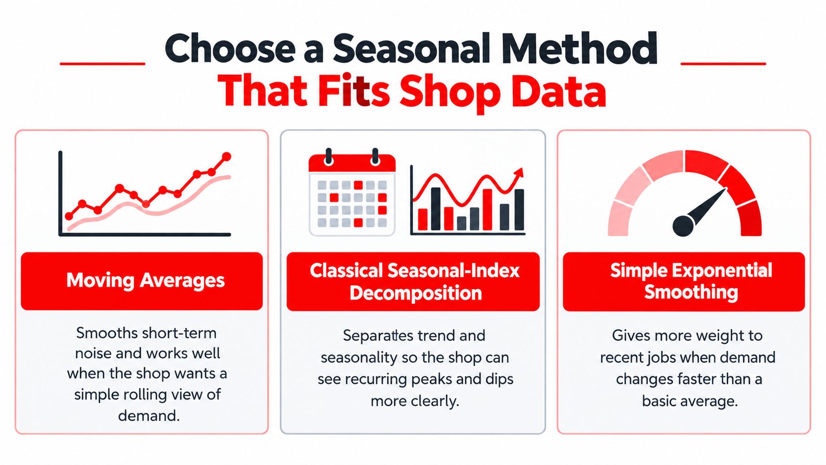
Three shop-ready methods cover most situations. The right pick depends on how much clean history exists and how regularly the category sells, not on which method sounds most advanced.
Compare the Three Options Honestly
Moving averages smooth short-term noise. A moving average taken over the length of the seasonal cycle becomes the baseline against which each period gets judged. It's the easiest starting point for a shop that wants a rolling view of demand and a reality check on whether volume is rising.
Classical seasonal-index decomposition goes one step further. The standard procedure divides each actual observation by that moving average, averages the factors for the same season across cycles, then multiplies a projected trend by the resulting index, as laid out in. Monthly data needs 12 monthly indices, and quarterly data needs four quarterly indices, per that same guide. This method suits categories with several comparable cycles, such as tires, batteries, cooling work, and inspections, because the recurring peak has repeated often enough to trust.
Simple exponential smoothing gives more weight to recent jobs. It fits short histories and categories where demand shifts faster than a plain average can follow. For sparse demand, shops should compare simple exponential smoothing, a moving average, TSB, and seasonal analogues rather than assuming a specialized intermittent method wins automatically.
That caution is earned. In, TSB and SESAP were the preferred combination, with SESAP restricted to seasonal items, while Croston and SBA performed worse than simpler methods such as SES or a moving average. A fancy label doesn't beat a clean, simple baseline.
Benchmark Before Trusting Any Pick
Every method should be tested against a naïve forecast and a seasonal-naïve forecast. The seasonal-naïve version repeats the same period from the last cycle, and it is embarrassingly hard to beat in strongly seasonal categories. If a chosen method can't outperform that, the method adds complexity without value.
Testing should use rolling-origin time-series cross-validation: train on an expanding historical window, forecast the next one or four weeks, record the error, and repeat across multiple seasonal cycles, following. Judging should rely on WAPE or MASE alongside RMSE, not MAPE alone, because values near zero create disproportionately large percentage errors. Low-volume categories punish MAPE and reward methods that look precise on paper while missing the week that matters.
The same discipline appears in other service businesses that staff against expected volume, and owners comparing approaches can see a parallel in efforts to. The trade differs, but the logic doesn't: expected demand drives scheduled hours.
The rule of thumb stays simple. Use the seasonal index when several comparable cycles exist. Use smoothing when the series is thin or irregular. Either way, seasonality shouldn't be treated as frozen, because instead of assuming every January or summer is identical. Patterns drift, and the method should allow that drift.
Run a Seasonal Index With Shop-Scale Numbers
A seasonal index is easier to trust after the arithmetic has been done once with plain numbers. The example below uses units, but shops can run the identical steps on repair orders, billed hours, or a single parts category.
Read the Index First
An index of 1.00 represents average demand, 1.30 represents demand 30% above average, and 0.64 represents demand 36% below average, according to. That single line tells a manager how far a given season sits from normal before any dollar figure enters the conversation.
Start with an annual average of 1,000 units, which gives a four-season average of 250 units per season in that same example. Multiply that baseline by each seasonal index and the flat average disappears. In shop terms, the high-index season might be winter batteries or summer cooling, while the low-index season is the quiet stretch where the schedule needs maintenance work and follow-up calls to stay full.
Seasonal Index Example From Annual Average to Period Forecast
| Season index | Demand at 1,000 annual units | Demand at 1,500 annual units |
|---|---|---|
| 1.16 | 290 | 435 |
| 0.64 | 160 | 240 |
| 0.90 | 225 | 337.5 |
| 1.30 | 325 | 487.5 |
The first forecast column comes straight from the example, where indices of 1.16, 0.64, 0.90, and 1.30 produce seasonal demands of 290, 160, 225, and 325 units. If projected average demand rises to 1,500 annually, the seasonal baseline becomes 375 per season, and the forecasts become 435, 240, 337.5, and 487.5 units. The math never changes: projected baseline multiplied by the index for that period.
Now compare that with staffing to a flat 250 or 375. The flat plan understaffs the peak season badly, because 325 or 487.5 units of demand can't fit into capacity built for an average period. It also overbuys and overstaffs the trough, where actual demand of 160 or 240 leaves paid hours with nothing to bill against.
A flat average is wrong in both directions. It starves the peak and wastes money in the dip.
Two cautions keep the index honest. One observed cycle isn't enough, because a single busy season could reflect a promotion, a recall, or unusual weather rather than repeatable seasonality. Any freak week already capped during data cleaning should stay out of the factor as well, since folding it back in rebuilds the distortion the cleaning step removed. The index earns trust only when the same pattern repeats across comparable cycles.
Turn the Forecast Into Hours Parts and Capacity
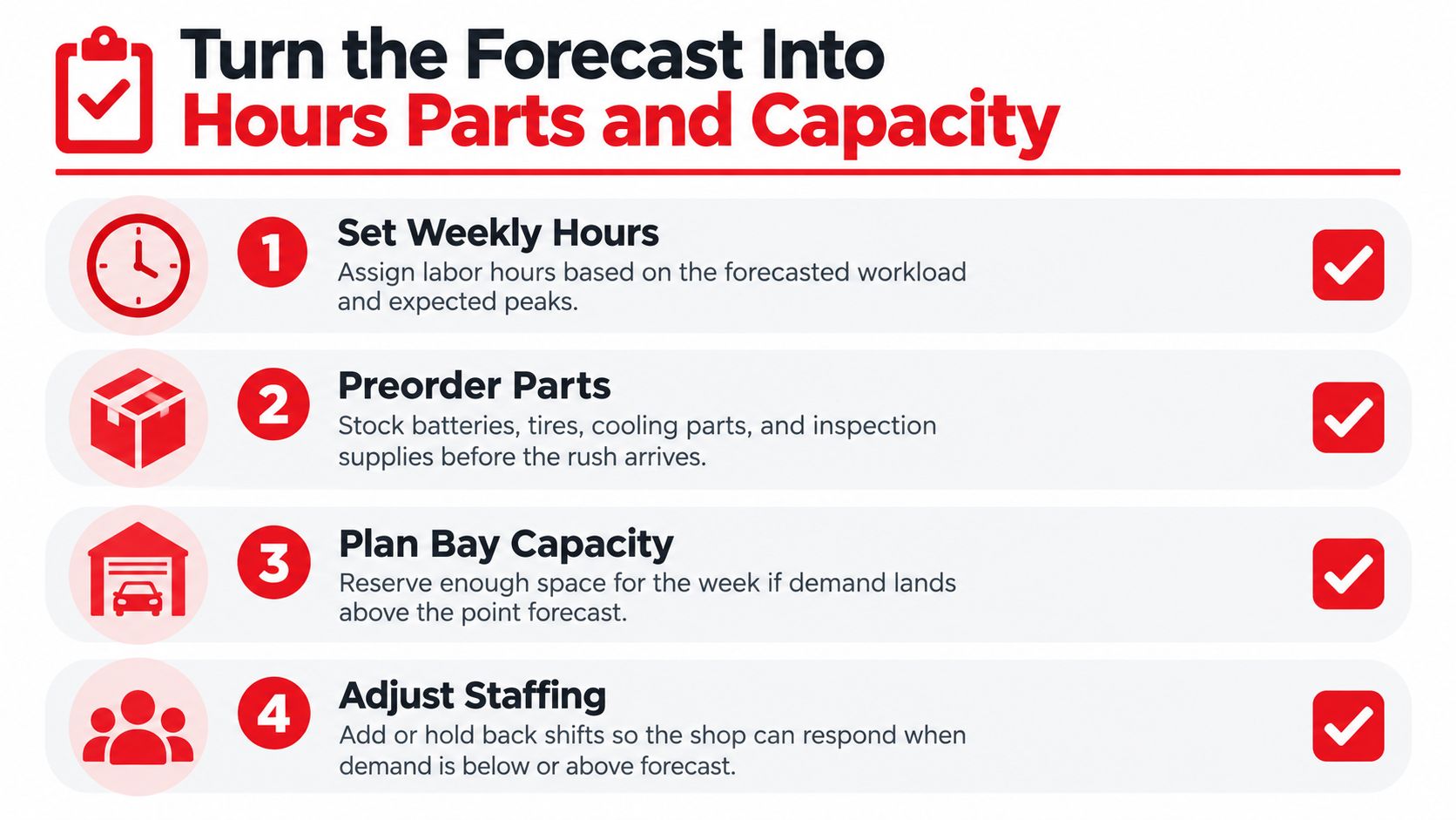
A weekly forecast becomes useful when it changes the schedule, parts order, or bay plan before the week starts. Convert each location's expected jobs into work hours and resources, then give the team a clear response for higher or lower demand.
Plan a Range, Not a Single Number
A job count is not a workload plan. Five inspections and five engine jobs take different technician-hours, bay time, and parts. For each week, estimate technician-hours, bay capacity, and parts replenishment targets. Use P50, P80, and P90 estimates to set a normal staffing level, a higher contingency level, and a parts target that accounts for stronger demand. Staff around the middle estimate and hold options for the high case, rather than paying overtime before you know the week will need it.
Forecast errors do not always follow a tidy pattern. A production-scheduling study found that probabilistic forecasts combined with stochastic optimization performed better than conventional approaches across 17 datasets and 303 products, and questioned the assumption that demand errors follow a Gaussian distribution. A small shop does not need that machinery. Write down best, base, and worst workload, including a practical case where demand comes in 20% above or below forecast.
- Base case: Schedule normal technician-hours and open the standard appointment book.
- High case: Hold contingency shifts, protect extra battery, tire, or cooling slots, and raise the parts buffer.
- Low case: Call customers about maintenance, fleet follow-ups, and deferred work to fill open bays.
Keep Location Plans Coherent
For a multi-location group, build the forecast at the most useful level: location by service type by week. Then reconcile those figures with each shop's plan and the network total. If local forecasts do not add up, locations can double-book parts or promise staffing the network cannot provide. Assign an owner to resolve those gaps before orders and schedules are set.
Treat intermittent work separately. Track how often a job appears and how large it is when it appears. A short run of zero-demand weeks does not prove the next week will also be zero. Keep a sensible parts and capacity plan for specialty work, so one arrival does not catch the shop unprepared.
RedAppy records already cover repair orders, real-time parts and supplier ordering, the team calendar, and analytics for revenue, technician efficiency, average repair order, and repeat business. Use the Digital Shop Board to check whether appointments are filling as forecast. Track service level and bias alongside statistical error. A good average error score can still hide repeated misses during the peak weeks that strain labor, bays, and parts.
Review Forecasts When Weather and Demand Shift
Last cycle's calendar pattern is a starting point, not a guarantee. Seasonal averages miss abrupt cold snaps, heat waves, storms, and strange transitions between seasons, and those events often drive the most profitable and most chaotic weeks of the year.
Separate the Baseline From the Event
Forecast skill becomes less deterministic beyond roughly two weeks, which calls for probabilistic views covering about two to six weeks and seasonal views covering one to six months, as described in. Shops should update with rolling weather information rather than waiting for the month to close. A neutral case using ECMWF seasonal forecasts and 51 weather scenarios improved winter consumption planning and clarified how extreme temperatures affect purchasing decisions, per that same overview.
The shop version of that idea is a trigger rule, not a new model. A temperature threshold or storm warning fires a defined response: add battery-testing slots, open winterization or cooling-system appointments, place a short parts replenishment order, and notify standby technicians. Owners setting the parts side of that response can work through buffer sizing with guidance to and then apply the result to batteries, tires, or cooling components.
After the event, the review matters as much as the response. The spike gets marked as event-driven demand so it doesn't get locked into next cycle's seasonal index as if it will repeat on schedule.
Re-estimate on a Rolling Basis
Forecasts should be refreshed regularly, with holiday markers kept current and each location's history kept separate. Patterns drift as vehicle fleets age, neighborhoods change, and service mixes shift. A forecast estimated once and left alone slowly becomes a description of a shop that no longer exists.
A short KPI set keeps the review focused:
- MASE or a similar scale-free error: Compares accuracy across categories with different volumes.
- Bias: Reveals systematic under-forecasting or over-forecasting.
- Range coverage: Shows whether high weeks landed inside the range the shop staffed to.
Reviews should also follow promotions, weather shocks, or bay constraints that changed what the shop could book. Observed demand during a constrained week understates true demand, and feeding it back unadjusted teaches the forecast to plan small. The two pitfalls worth naming are optimizing average error while the costly peak stays wrong, and fitting a complex model to a single season. A more elaborate model is not automatically the fix. Trigger rules and honest ranges usually beat false precision.
Put Seasonal Demand Forecasting to Work This Week
By Friday, you should have a forecast that changes next week's schedule. Keep the first version small, use it to set bay hours and parts buffers, then improve it as more shop history comes in. A simple forecast on the schedule beats a polished model left in a spreadsheet.
A First-Week Action List
- Choose two or three seasonal categories. Start with batteries, tires, cooling, or inspections, where a shift in demand affects bays and parts.
- Export weekly history. Pull repair orders by category and week. Flag unusual demand, promotions, and closure weeks.
- Set a baseline. Use a seasonal index when cycles repeat; use smoothing when the history is thin.
- Plan three outcomes. For each, estimate technician-hours and the buffer for one key parts category.
- Set a review time. Check the forecast after each busy week and whenever a weather trigger fires.
Limited history is no reason to wait. 12 validated months can get a shop started, though a stronger seasonal estimate may require 24 to 36 months of history. With fewer cycles, choose a simpler method and allow wider forecast ranges. Regional patterns and supplier lead times can help fill gaps while the shop builds its own weekly record.
The payoff is practical: bays staffed for the rush, parts on hand, and advisors able to accept seasonal work. Give the forecast a regular place in shop operations. Review scheduling, repair-order history, parts ordering, and shop analytics on the RedAppy features page, or discuss using existing shop records for a weekly forecast by contacting the RedAppy team. Repair-order records already capture the work moving through the shop, from first call to final payment. Use them to plan peak weeks before the schedule fills.
Turn next season's rush into a staffed, stocked plan with repair-order history, scheduling, parts ordering, and shop analytics working from the same records. Visit RedAppy to see how seasonal demand forecasting fits the daily flow from first call to final payment and start planning peak weeks before they arrive.
Ready to Transform Your Shop?
RedAppy helps auto repair shops create professional digital estimates with photos and videos, send them instantly via text or email, and get customer approvals in seconds. No credit card required to start.